
Upcoming webinar on 'Inforiver Charts : The fastest way to deliver stories in Power BI', Aug 29th , Monday, 10.30 AM CST. Register Now
Upcoming webinar on 'Inforiver Charts : The fastest way to deliver stories in Power BI', Aug 29th , Monday, 10.30 AM CST. Register Now
Understanding data patterns in scatter and bubble charts can often require more than just visual interpretation. This is where trendlines play a critical role. Inforiver Analytics+ includes built-in support for trendlines as part of its advanced analytics capabilities, enabling users to overlay predictive insights directly on their visualizations. With options to display both the trendline equation and R² value, these features help finance, planning, and data analytics professionals assess data relationships and model performance more effectively.
In this blog post, we explore the different types of trendlines available, how to select the most appropriate one for your dataset, and key use cases that drive better business decisions.
Trendline is a line superimposed on top of your chart that helps you reveal the underlying patterns. This makes it easier to forecast outcomes and support strategic decisions. It is essentially part of a statistical analysis model which helps exploring relationships between two or more variables.
The most common multi-variable chart is Bubble/Scatter chart. It allows you to plot 2 to 3 variables simultaneously. Inforiver Analytics+ offers Bubble/Scatter chart family, which includes scatter plot, bubble plot, and quadrant plot. It supports all the advanced features such as conditional formatting, dynamic marker size, shape, drill down, and analytical lines.
Inforiver analytics+ offer multiple types of trendlines, each suited for specific data behaviour:
Note - Moving Average: This isn't a trendline but rather a smoothing technique. It calculates the average of data points over a specified period, helping to smooth out short-term fluctuations and reveal the underlying trend.
| Linear Trendline | Exponential Trendline | Logarithmic Trendline | Polynomial Trendline | |
| Appearance | A straight diagonal line | A curve rising steeply upward | A curve rising then flattening | A U-curve or S-curve |
| Definition | Shows a constant rate of change between two variables, modelling direct, proportional relationships. | Models rapid, compounding growth. Useful for markets where performance increases significantly after a certain threshold. | Fits data that starts fast and then slows down. Helps detect saturation or over-investment limits in high-population markets. | Captures trends with peaks, valleys, or inflection points. Great for identifying optimal performance zones or behavior changes. |
| Equation Type | y=mx+b | y=a⋅ebx | y=a⋅ln(x)+b | y=ax²+bx+c |
| What It's Best For | Understanding baseline correlation between variables | Spotting acceleration in high-growth or tipping-point markets | Highlighting diminishing returns with growth | Exploring complex, non-linear relationships |
| Key Idea | Simple and clear relationship—more sales equals more quantity. | Growth keeps increasing faster over time. | Big early gains, slower long-term growth. | Performance varies across the spectrum. |
| When to Use | Use when the relationship between two variables is steady and predictable. | Use when data accelerates quickly—e.g., startup growth, viral trends, large population markets. | Long-term growth. Use when initial performance is strong but later gains taper off—e.g., mature markets or platforms. | Use when data doesn’t follow a simple pattern—e.g., small vs. mid vs. large city comparisons. |
Real world example: City-wise Sales Performance
Let’s illustrate how different trendlines can tell different stories using a bubble chart of city-wise sales performance.
Bubble Chart displays data for various cities, with:
Refer to the below image where cities like New York, Los Angeles, and Chicago appear in the upper-right quadrant, indicating strong performance in both sales and quantity sold, while cities like Denver or Washington cluster in the lower-left, showing relatively lower metrics.
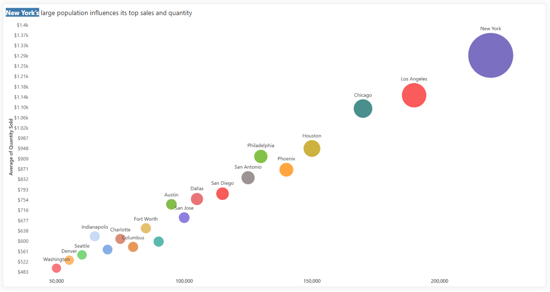
Figure 1: Bubble/Scatter Chart
Use Case: Understanding baseline correlation between sales and quantity sold.
In a bubble or scatter chart where sales are plotted on the X-axis and quantity sold on the Y-axis, a linear trendline helps establish the general relationship between these two metrics. Typically, as sales increase, quantity sold also increases—indicating a positive linear correlation.
The linear trendline is represented by the equation:
y=mx+b
Where:
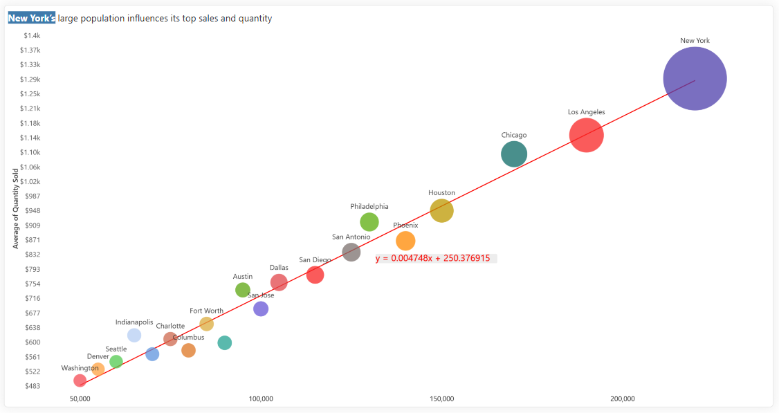
Figure 2: Bubble/Scatter Chart - Linear Trendline
Use Case: Spotting acceleration in high-growth markets
An exponential trendline is best used when data shows a consistent rate of increase that becomes more rapid over time—indicating compounding growth. In the context of city-level data, this trendline can reveal how sales and quantity sold increase disproportionately in larger, more populated cities. This suggests that once a city crosses a certain population threshold, market activity may accelerate significantly, signalling a “tipping point” for potential investment.
The Exponential trendline is represented by the equation:
y=a⋅ebx
Where:

Figure 3: Bubble/Scatter Chart - Exponential Trendline
Use Case: Highlighting diminishing returns with growth
A logarithmic trendline is ideal when growth increases quickly at first but slows down as it progresses—reflecting diminishing returns. Applied to city-level sales data, this trendline might show that while sales initially rise sharply with population, the gains taper off in larger cities. This insight helps decision-makers understand where additional investment may yield limited returns, especially in saturated or mature markets.
The Logarithmic trendline is represented by the equation:
y=a⋅ln(x)+b
Where:
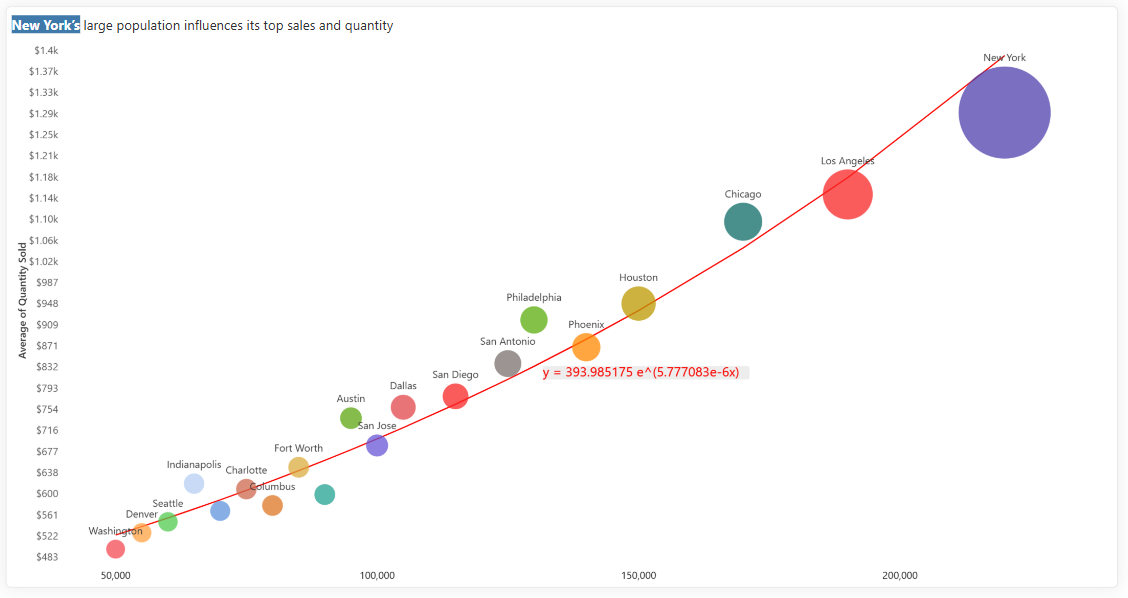
Figure 4: Bubble/Scatter Chart - Logarithmic Trendline
Use Case: Exploring complex relationships across city sizes
A polynomial trendline is suited for data that follows a non-linear, curved pattern—helping capture more nuanced behaviors. In the context of city performance, it may reveal that mid-sized cities outperform both very large and very small ones, possibly due to better cost-efficiency or operational balance. This makes it a powerful tool for uncovering high-performance zones in the market.
The Polynomial trendline is represented by the equation:
y=ax²+bx+c
Where:
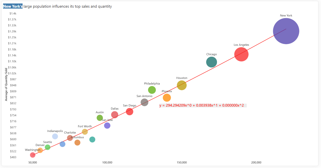
Figure 5: Bubble/Scatter Chart - Polynomial Trendline
While the equation form gives you insight into the type of relationship, the R-squared value (R2) is crucial for determining how well that equation fits your data.
Trendlines are powerful analytical tools that highlight insights. By understanding the different types of trendlines and how to interpret their equations and R-squared values, you can uncover hidden patterns, forecast future trends, and make more informed strategic decisions. Whether you're analyzing sales performance, market growth, or any other data set, mastering trendlines will empower you to tell compelling data stories and drive better outcomes for your business.
Start exploring your data with trendlines today and try Inforiver Analytics+ for free!

Inforiver helps enterprises consolidate planning, reporting & analytics on a single platform (Power BI). The no-code, self-service award-winning platform has been recognized as the industry’s best and is adopted by many Fortune 100 firms.
Inforiver is a product of Lumel, the #1 Power BI AppSource Partner. The firm serves over 3,000 customers worldwide through its portfolio of products offered under the brands Inforiver, EDITable, ValQ, and xViz.
 Learn how to build advanced, insight-rich Power BI dashboards effortlessly with Inforiver Analytics+—no coding, no complex configurations, just smarter reporting in less time.