Upcoming webinar on 'Inforiver Charts : The fastest way to deliver stories in Power BI', Aug 29th , Monday, 10.30 AM CST. Register Now
Upcoming webinar on 'Inforiver Charts : The fastest way to deliver stories in Power BI', Aug 29th , Monday, 10.30 AM CST. Register Now
Do users complain about slow loading times and unresponsive dashboards? A sluggish report can be a major roadblock.
The good news is you don't have to live with slow performance. By applying a few strategic best practices, you can dramatically improve the speed and efficiency of your Power BI reports.
This guide breaks down 30 key practices across six crucial areas, giving you the tools to build reports that are not only powerful but also lightning-fast.
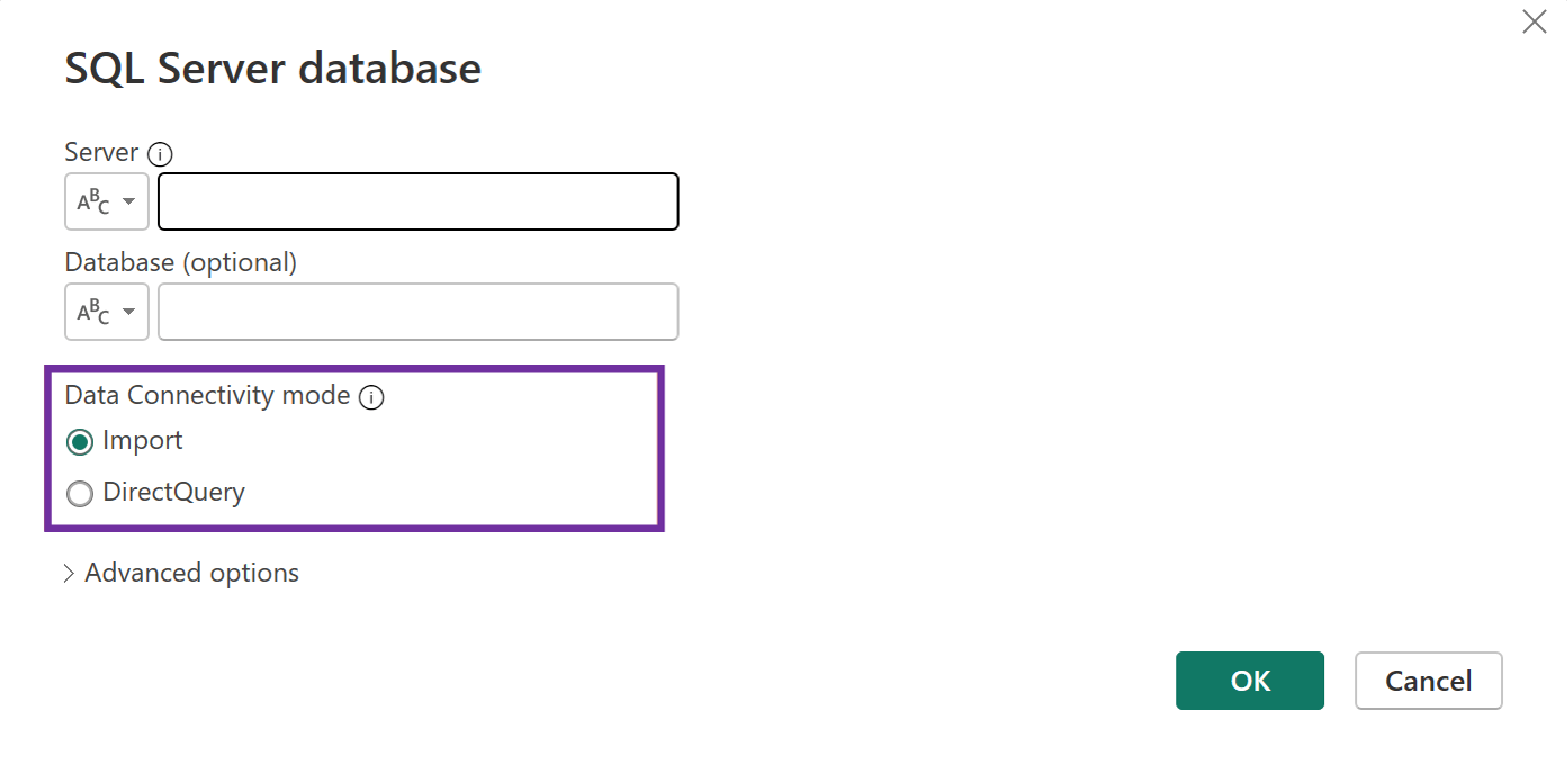
The foundation of a high-performance report starts with how you connect to your data.
Understanding the backend mechanics here is critical.
Ever wonder why some dashboards feel lightning-fast while others leave you waiting?
The secret often lies in Import Mode. Instead of constantly running back to your source data, Power BI creates a local, super-fast copy.
This copy lives in a special in-memory database called the VertiPaq engine. The VertiPaq engine uses a clever technique called columnar storage and advanced compression, which makes your data model smaller and allows visuals to respond almost instantly, even with millions of rows.
It also gives you access to the full suite of Power Query and DAX tools.
Unlike Import Mode, DirectQuery acts as a live link to your data source.
This is perfect for when you need real-time data or are working with a massive dataset that’s simply too big to fit in memory. However, performance is entirely dependent on the speed of your source database.
This means optimizing DirectQuery is about optimizing the source itself. Work with your database administrators to ensure columns used for filtering and joining are indexed and consider creating materialized views or pre-aggregated tables to offload heavy computations from the report to the database.
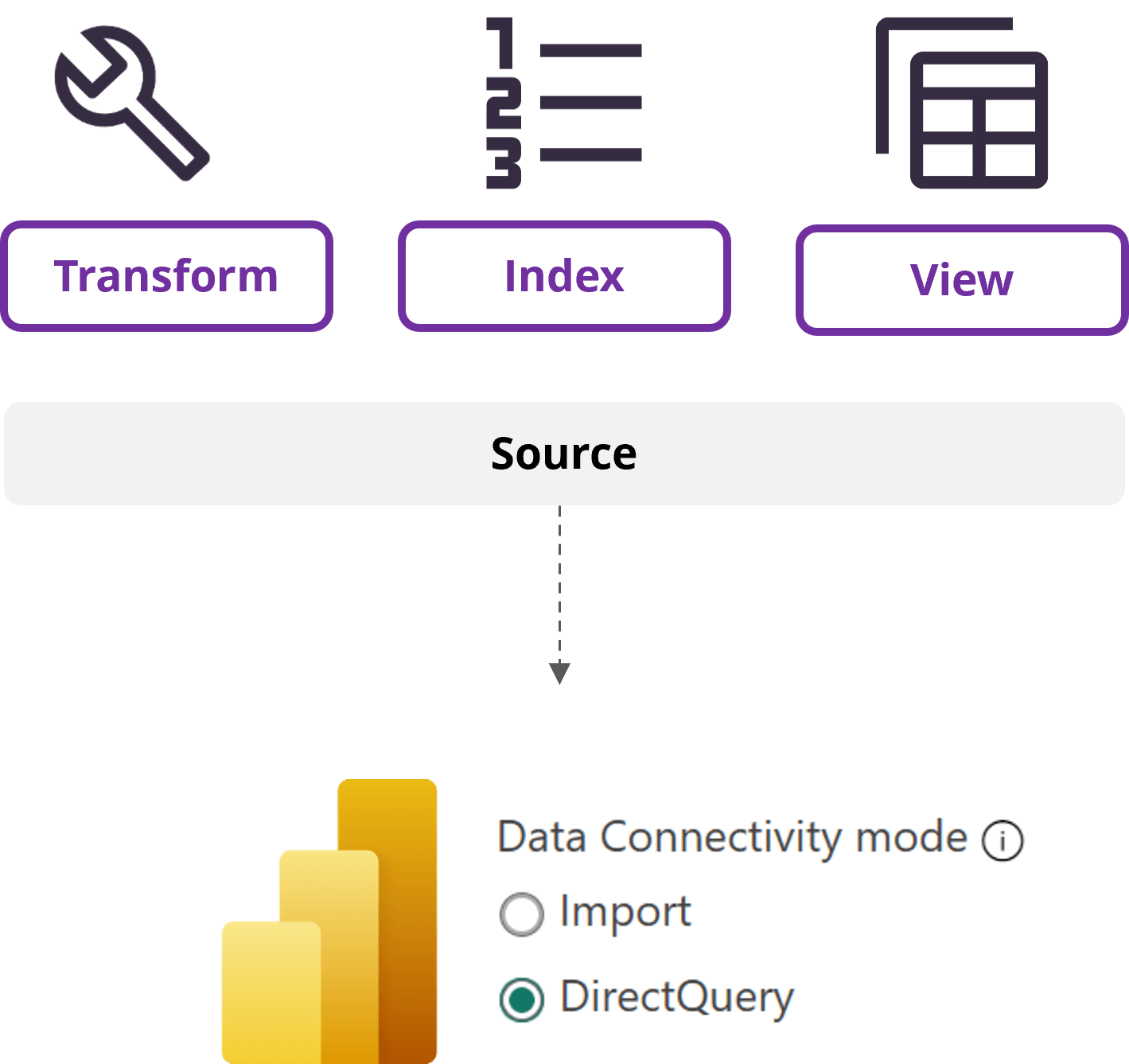
A blend of Import and DirectQuery.
Hybrid Tables use partitions: a fast, historical partition in Import Mode and a real-time partition in DirectQuery.
This gives you the best of both worlds. For Microsoft Fabric users, Direct Lake is a revolutionary approach that bypasses data movement altogether, reading data directly from Delta Parquet files in OneLake and giving you real-time data with Import-like performance.

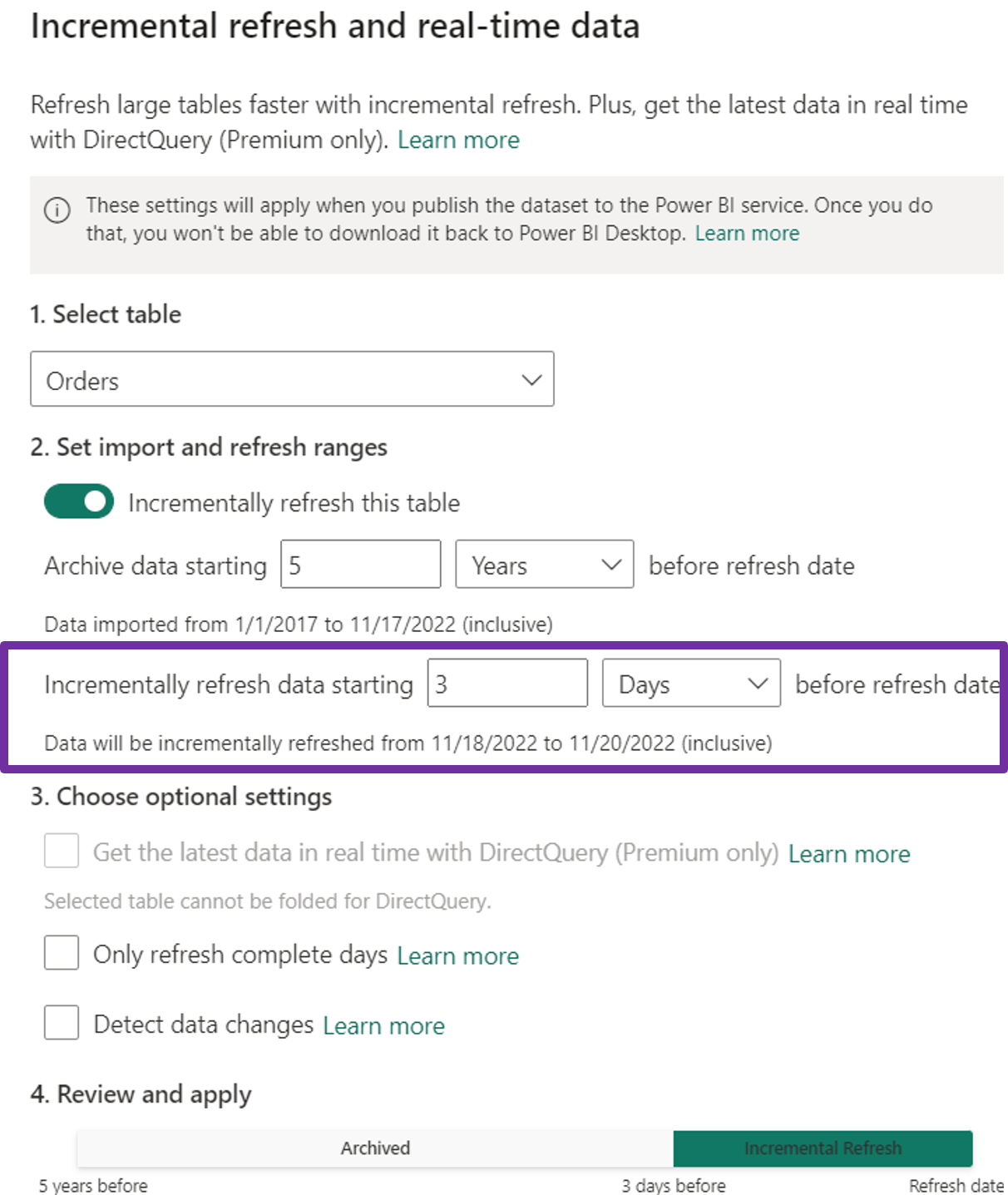
For large Import Mode datasets that grow over time, incremental refresh is a game-changer. Instead of reloading the entire table during each refresh, Power BI only updates a small, recent portion of the data.
This significantly reduces refresh time and resources. The magic lies in data partitioning, where you define a policy based on a date column, ensuring only the most recent data is processed while older partitions remain untouched.
The data model is the bedrock of your report.
A well-designed model is the single most important factor for achieving optimal performance.
The VertiPaq engine is optimized for a star schema design, with one central fact table containing numerical values (your measures) and several surrounding dimension tables with descriptive attributes (your slicers and filters).
The star schema's flat dimension tables reduce the number of joins needed to get your data. Since VertiPaq can perform these joins on compressed, single-column lookups, queries are executed with incredible speed.
By having a few, wider dimension tables rather than many small, linked ones (like in a snowflake schema), the VertiPaq engine can apply its compression algorithms more effectively, making your data model smaller and faster.

It is highly recommended to use unique, system-generated identifiers (often integers) in dimension tables. These ensure a unique key for establishing relationships, particularly when natural keys are not unique, are composite, or might change over time. Power Query's index column feature can be instrumental in creating these surrogate keys. The VertiPaq engine's compression algorithms, especially dictionary encoding, work most efficiently on low-cardinality integer columns.
Using a single, clean integer key for relationships is far more performant than joining on multiple text columns or complex natural keys.

This technique simplifies your model by consolidating multiple low-cardinality flags and attributes into a single table. This reduces clutter and the overhead of managing multiple small dimension relationships.
These tables contain only dimension keys and no numerical measures. They are useful for measuring events where there's no numerical value to aggregate (e.g., student attendance). In the backend, they are extremely lean as they only need to store compressed integer keys.
A fundamental principle for high-performance Power BI models is to load only the data that is necessary for the intended analysis. Smaller models lead to faster data refresh cycles, consume less memory, and enable quicker query responses.
This is a primary defense against exceeding memory limits and experiencing performance degradation, especially with the VertiPaq engine. The less data VertiPaq must scan, compress, and retain in memory, the more efficiently it operates.
The effectiveness of VertiPaq's compression algorithms is directly enhanced by data reduction fewer distinct values in columns, achieved by removing irrelevant data or high-cardinality columns, result in better compression ratios.
Eliminate unnecessary columns and rows as early as possible. A huge performance gain comes from disabling the "Auto Date/Time" option and using a single, centralized date dimension table instead, which prevents significant model bloat.
A simple one-to-many relationship with a single filter direction is highly efficient.
This feature should be used with caution as it can introduce ambiguity in filter paths, potentially leading to circular dependencies that the engine must resolve, which can negatively impact performance and make the model harder to understand and debug.
Bi-directional filtering is sometimes necessary for specific analytical requirements, such as enabling a slicer based on a fact table to filter another fact table through a shared dimension, or for certain Row-Level Security (RLS) implementations.
The Power BI engine's default behaviour with single-direction filtering is highly optimized for star schemas introducing bi-directional filters should be a deliberate design choice for specific, well-understood scenarios rather than a default approach.

A critical aspect of data modelling in Power BI involves understanding the distinction between calculated columns and measures, as their behaviour and performance characteristics are fundamentally different.
Calculated Columns
Measures
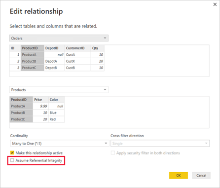
This setting is available for one-to-many and one-to-one relationships between two DirectQuery storage mode tables that belong to the same source group.
If enabled, and if the "many" side column of the relationship is guaranteed not to contain NULL values and referential integrity is maintained by the source database (e.g., through foreign key constraints), Power BI can generate more efficient source queries using INNER JOIN operations instead of OUTER JOIN operations.
An INNER JOIN is typically faster as it only returns rows where there is a match in both tables. However, enabling ARI when data integrity is not actually guaranteed can lead to silently incorrect results, as rows with foreign keys that do not exist in the dimension table will be dropped by the INNER JOIN, resulting in understated totals.
An OUTER JOIN would preserve these fact rows, showing NULLs for the dimension attributes. Thus, ARI presents a trade-off between potential speed gains and the risk of data inaccuracy, underscoring the importance of robust data governance and quality assurance processes before enabling this feature.
Power Query is where your data comes to life. Optimizing your M code here is essential for fast refresh times.
Query folding is a critical Power Query feature where the transformations defined in the M language are translated into the native query language of the underlying data source (e.g., SQL for relational databases) and executed directly by that source system. This "pushdown" of operations offers substantial performance benefits.
The source system processes the transformations and returns only the resultant, often smaller, dataset to Power BI. This minimizes the volume of data transferred over the network.
Leveraging the processing power of the source database (which is often optimized for such operations) can be significantly faster than pulling raw data into Power BI's mashup engine for transformation.
Less data processing by the Power BI mashup engine means lower CPU and memory consumption on the gateway (for on-premises sources) or the Power BI service.
You can check if folding is occurring by right clicking a step and selecting "View Native Query.

Not all M functions can be translated into a native query. Functions that require the entire dataset to be loaded into memory (like sorting on a non-indexed column) will "break" query folding.
The best practice is to perform folding-friendly steps (like filtering rows and removing columns) early in the query before any folding-breaking steps.
Data types directly affect the VertiPaq engine's compression. Numeric and Boolean data types are far more compressible than text.
Using the right data type ensures the most efficient compression, leading to a smaller model and faster query execution. Data types should be defined as early as possible in the Power Query transformation sequence, ideally in the "Source" step or immediately thereafter if the source doesn't provide clear type information.
Do not rely on Power BI's automatic type detection for all columns, as it may not always choose the most optimal type.
The VertiPaq engine is optimized for date data. Storing a date/time column when you only need the date part adds unnecessary overhead and increases the number of unique values (cardinality), which is bad for compression.
By splitting these columns in Power Query, you reduce cardinality, which improves compression and query speed.

If you use helper queries to clean and prepare data before it is merged into a final table, you can disable "Enable load" for these queries.
This prevents the M engine from loading them into the VertiPaq model, keeping your model size down and ensuring only the final, clean tables are available for reporting.
DAX is the language of your measures. The way you write DAX can be the difference between a sub-second response and a long wait.
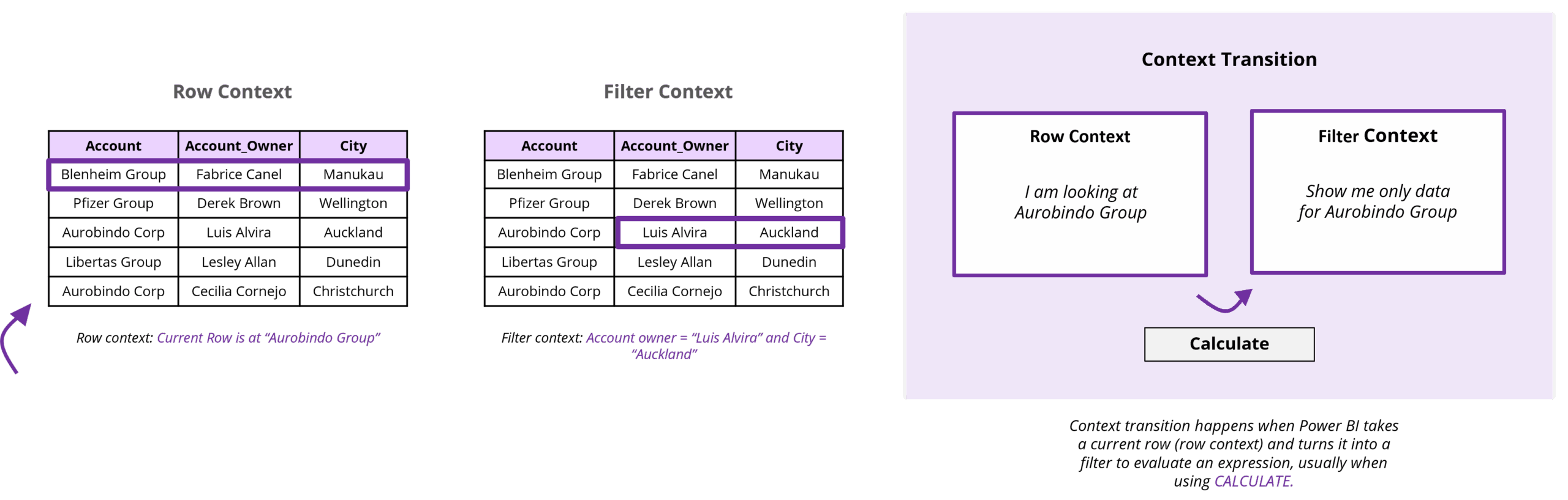
This is a crucial concept that occurs when a measure (which operates in a filter context) or a direct table reference is used within an existing row context (e.g., inside an iterator function like SUMX, or within the formula of a calculated column that calls a measure).
During context transition, the current row context is transformed into an equivalent filter context. This new filter context includes filters for all column values from the current row of the table being iterated over.
While context transition is a powerful mechanism enabling complex calculations, it can also be computationally expensive if it occurs frequently, especially within nested iterations or over large tables.
Optimizing DAX often involves refactoring formulas to minimize the number and depth of context transitions, perhaps by using variables to store values before entering an iteration or by redesigning the logic to rely more on set-based operations.
The performance difference between using the FILTER function as a simple table iterator versus using filter conditions directly as arguments to CALCULATE (often referred to as CALCULATE modifiers) can be substantial.
Functions like SUM, AVERAGE, and COUNT are simple, set-based functions that can be fully optimized by the Storage Engine.
Iterators like SUMX and AVERAGEX force the Formula Engine to iterate row-by-row, which is a much slower process. Wherever possible, use the simple aggregators.
variables, defined in DAX using the VAR... RETURN syntax is a cornerstone of writing efficient, readable, and maintainable DAX formulas.
By ensuring that a specific expression is evaluated only once, variables prevent the DAX engine from repeatedly executing potentially complex or resource-intensive logic, which can lead to dramatic reductions in query execution times.
The resulting value is then stored and can be reused multiple times throughout the remainder of the RETURN clause of that formula without incurring the cost of re-computation. This is particularly crucial for expressions that are computationally expensive or are referenced multiple times within conditional logic
The choice of DAX function matters. For example, DIVIDE is a better choice than the / operator because it handles division-by-zero errors gracefully and more efficiently. COUNTROWS is an optimized function that is faster than iterating through rows yourself.
| Less Performant / Risky Pattern | Safer & More Performant Alternative | Why It's Better |
|---|---|---|
| [Numerator] / [Denominator] | DIVIDE([Numerator], [Denominator], 0) | Gracefully handles division by zero errors and is more efficient. |
| COUNT([ColumnName]) | COUNTROWS( | Directly counts all rows in a table, which is faster than counting non-BLANK values in a column. |
| IF(HASONEVALUE(Table[Column]), VALUES(Table[Column]), "N/A") | SELECTEDVALUE(Table[Column], "N/A") | A more concise and efficient function for retrieving a single selected value from a column. |
| FILTER(Table, Condition) in CALCULATE | CALCULATE(Expression, Table[Column] = "Value") | Using direct Boolean conditions as CALCULATE modifiers is more efficient than creating an intermediate filtered table. |
| ALL(TableOrColumn) to respect visual filters | ALLSELECTED(TableOrColumn) | Respects filters applied by slicers and other visuals, resulting in more accurate and efficient calculations within a given visual context |
| IFERROR(Expression, Value) | DIVIDE or preventative logic | Generic error functions can force less-efficient row-by-row evaluation. It's better to use specific functions like DIVIDE |
Returning BLANK is often more efficient than returning 0 in DAX.
The VertiPaq engine is highly optimized for storing BLANK values, so returning them does not add significant overhead.
This also helps visuals display only meaningful data, reducing rendering complexity and improving the user experience.
Even with a perfect data model, a poorly designed report can be slow. Here’s how to make the frontend as fast as the backend.
One of the most common culprits of slow report pages is an excessive number of visuals. Each visual element on a report page, whether it displays data or is purely decorative, contributes to the overall load time. Each data-bound visual typically sends one or more queries to the data model and then requires time to render its output. The cumulative effect of many visuals, even simple ones, can lead to significant performance degradation, a phenomenon sometimes described as "death by a thousand cuts."
A general guideline suggested by some experts is to aim for a maximum of 5-10 data-driven visuals per page, including KPI cards. Allow users to navigate from a summary visual to a more detailed report page, filtered to the context of the selected data point.
Configure custom tooltips that appear when a user hovers over a data point in a visual. These tooltips can be entire report pages themselves, displaying additional contextual visuals and information.
Complex visuals with a high number of data points, intricate conditional formatting, or custom styling can strain the rendering engine. Use filters like "Top N" to reduce the number of data points. For example, a bar chart with 10 categories will be significantly faster to render than one with 10,000.
While conditional formatting can enhance data interpretation, excessive or highly complex conditional formatting rules applied to visuals can add significant query overhead and slow down rendering, as each rule may need to be evaluated for numerous data points.
Custom visuals from AppSource can be a double-edged sword. While they offer specialized functionality, their performance is not guaranteed to be as optimized as native Power BI visuals. They can often generate less-efficient DAX queries or have slower rendering engines. Always benchmark a custom visual before deploying it.

Slicers are the most common source of "query chatter."
Every time a user interacts with a slicer, it sends a new DAX query for every visual on the page. For heavy reports, consider using the "Apply button" for slicers to batch filter changes and prevent a cascade of queries. Also, use the "Edit Interactions" feature to prevent visuals from unnecessarily cross-filtering each other.
We suggest SuperFilter with smooth performance for larger datasets (Up To ~150k rows). It improves report load time and eliminates slicer lag.

Performance optimization isn't a one-time task; it's a continuous journey. You need the right tools to monitor and troubleshoot issues as they arise.
This built-in tool is your window into the query backend. It shows you the DAX query generated by each visual and breaks down the time it took to execute. This allows you to directly identify which visuals and which DAX expressions are causing bottlenecks.
When recording is started, the Performance Analyzer logs the time taken by each visual on a report page to execute its DAX queries, render the visual display, and perform other operations (like waiting for other visuals or preparing queries). This occurs when the page is initially loaded or when users interact with slicers or other report elements.

For a deeper dive, DAX Studio is an external tool that lets you run and analyse DAX queries directly against the VertiPaq engine. It can show you the query plan and server timings. DAX Studio can connect directly to Power BI Desktop models or to datasets hosted in the Power BI service (via the XMLA endpoint for Premium/PPU workspaces).
For DirectQuery, SQL Server Profiler can be used to monitor the native queries being sent to the source database.
In a Premium or Fabric capacity, you have access to a Capacity Metrics app that shows the overall resource consumption of your reports. You can monitor CPU usage, memory consumption, and query execution times to identify reports that are a strain on the entire environment.

When a report is slow, a systematic approach is more effective. Start with the basics: Is the data source slow? Is the gateway overloaded? Then, use the Performance Analyzer to find the slowest visuals. From there, use DAX Studio to optimize the DAX queries. Finally, check your data model and Power Query steps. This methodical approach will prevent you from making random changes.
Identify Scope and Context: Before you do anything else, figure out the basics. Is the report slow all the time, or just at specific moments? Is the slowness affecting everyone or only a few users? Knowing the context will point you in the right direction.
Premium/Fabric Capacity Investigation: If your report is hosted on a Premium or Fabric capacity, check the Capacity Metrics app first. This will tell you if the capacity is under pressure due to resource exhaustion (like high CPU or memory usage).
Shared Capacity Investigation: If you're not on Premium, you're on a shared capacity. In this case, your primary tool is the Power BI Performance Analyzer in Power BI Desktop. This will help you pinpoint whether the bottleneck is in the DAX queries or the visual rendering.
Gateway and Data Source Checks: Investigate the data connection. Is the on-premises data gateway overwhelmed? Is the source database itself running slowly? Use tools like SQL Server Profiler to see what's happening at the source.
Consider Architectural Changes: If the above steps don't fix the issue, you might need to make bigger changes. This could involve using a Composite model, migrating to a Premium capacity, or optimizing your data source architecture.
Iterate and Validate: Performance tuning is a cycle. After you apply an optimization, always re-test using the Performance Analyzer to confirm that your change had the desired effect.
Raise Support Ticket: If you've gone through all the steps and the issue persists, it's time to contact Microsoft support. Provide them with all the details you've gathered from your systematic investigation.


Inforiver helps enterprises consolidate planning, reporting & analytics on a single platform (Power BI). The no-code, self-service award-winning platform has been recognized as the industry’s best and is adopted by many Fortune 100 firms.
Inforiver is a product of Lumel, the #1 Power BI AppSource Partner. The firm serves over 3,000 customers worldwide through its portfolio of products offered under the brands Inforiver, EDITable, ValQ, and xViz.